Explain Different types of Sampling Techniques

Sampling Techniques

Basically, there are three types of sampling techniques such as:

(i) Instantaneous sampling

(ii) Natural sampling

(iii) Flat top sampling

Out of these three, instantaneous sampling is called ideal sampling whereas natural sampling and flat-top sampling are called practical sampling methods.

Now, let us discuss three different types of sampling techniques in detail.

(i) Instantaneous sampling

In this type of sampling, the sampling function is a train of impulses. Fig.1(b) shows this sampling function.

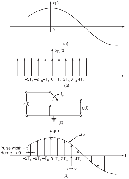
Fig.1 : (a) Baseband signal, (b) impulse train, (c) functional diagram of a switching sampler, (d) sampled signal

x(t) is the input signal (i.e., signal to be sampled) as shown in fig.1(a).

Fig.1(c) shows a circuit to produce instantaneous or ideal sampling.This circuit is known as the switching sampler.

The working principle of this circuit is quite easy. The circuit simply consists of a switch. Now if we assume that the closing time ‘t’ of the switch approaches zero, then the output g(t) of this circuit will contain only instantaneous value of the input signal x(t).

Since the width of the pulse approaches zero, the instantaneous sampling gives a train of impulses of height equal to the instantaneous value of the input signal x(t) at the sampling instant.

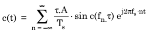
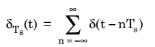
We know that the train of impulses may be represented as,

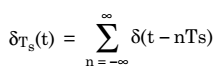
This is known as sampling function and its waveform is shown in fig.1(b).

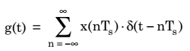
The sampled signal g(t) is expressed as the multiplication of x(t) ans δT_s(t). Thus,

Or

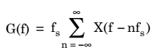
The Fourier transform of the ideally sampled signal given by above equation may be expressed as,

Natural Sampling

As we have already discussed, the instantaneous sampling results in the samples whose width τ approaches zero. Due to this, the power content in the instantaneously sampled pulse is negligible. Thus, this method is not suitable for transmission purpose.

Natural sampling is a practical method. In this type of sampling, the pulse has a finite width equal to τ.

Let us consider an analog continuous-time signal x(t) to be sampled at the rate of f_s Hertz.

Here it is assumed that f_s is higher than Nyquist rate such that sampling theorem is satisfied.

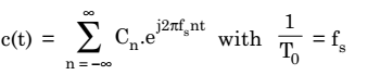
Again, let us consider a sampling function c(t) which is a train of periodic pulses of width τ and frequency equal to f_s Hz.

Fig.2 shows a functional diagram of a natural sampler.

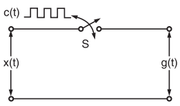
Fig.2 : A functional diagram of a natural sampler

With the help of this natural sampler, a sampled signal g(t) is obtained by multiplication of sampling function c(t) and input signal x(t).

Now, according to fig.2, we have when c(t) goes high, the switch ‘S’ is closed. Therefore,

g(t) = x(t) when c(t) = A

g(t) = 0 when c(t) = 0

where A is the amplitude of c(t).

The waveforms of signals x(t), c(t) and g(t) have been illustrated in fig.3(a), (b) and (c) respectively.

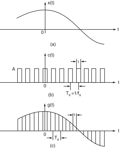
Fig.3 : (a) Continuous time signal x(t), (b) Sampling function waveform i.e., periodic pulse train, (c) Naturally sampled signal waveform g(t)

Now, the sampled signal g(t) may also be described mathematically as

g(t) = c(t) . x(t)

Here, c(t) is the periodic train of pulse of width t and frequency f_s.

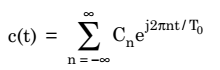
We know that the exponential Fourier series for any periodic waveform is expressed as,

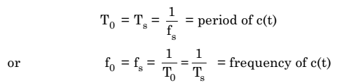
Also, for the periodic pulse train of c(t), we have,

So, we have

Now, it may be noted that since c(t) is a rectangular pulse train, therefore C_n for this waveform will be expressed as,

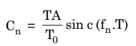
here T = pulse width = τ

and fn = harmonic frequency

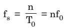
But here, f_n = nf_s

or,

Hence,

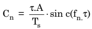
Therefore,  the Fourier series representation for c(t) will be given as,

Now, substituting the value of c(t) in the equation of g(t), we get,

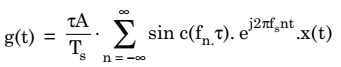
This is required time-domain representation for naturally sampled signal g(t).

Now, to get the frequency-domain representation of the naturally sampled signal g(t), let us take its Fourier transform as,

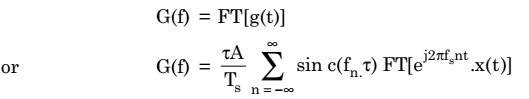
Recall the frequency-shifting property of Fourier transform which states that

Therefore,

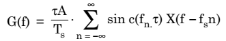
Now, since f_n = nf_s = harmonic frequency

Therefore,

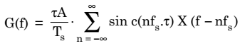
Hence, we write Spectrum of naturally sampled signal:

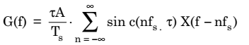
This equation shows that the spectra of x(t) i.e., X(f) are periodic in f_s and are weighed by the sinc function.

Fig.4 illustrates some arbitrary spectra for x(t) and corresponding spectrum G(f).

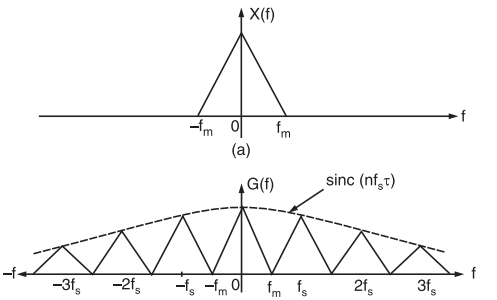
Fig.4 :(a) Spectrum of continuous-time signal x(t), (b) Spectrum of naturally sampled signal

Flat Top Sampling or Rectangular Pulse Sampling

Flat top sampling like natural sampling is also a practically possible sampling method. But natural sampling is little complex whereas flat top sampling is quite easy.

In flat-top sampling or rectangular pulse sampling, the top of the samples remains constant and is equal to the instantaneous value of the baseband signal x(t) at the start of sampling.

The duration or width of each sample is τ and sampling rate is equal to f_s = 1 / T_s.

Fig.5(a) shows the functional diagram of a sample and hold circuit which is used to generate the flat top samples.

Fig.5 :(a) A sample and hold circuit to generate flat top samples (b) A general waveform of flat top sampling

Fig. 5(b) shows the general waveform of flat top samples. From fig.5(b), it may be noted that only starting edge of the pulse represents instantaneous value of the baseband signal x(t).

Also the flat top pulse of g(t) is mathematically equivalent to the convolution of instantaneous sample and a pulse h(t) as depicted in fig.6.

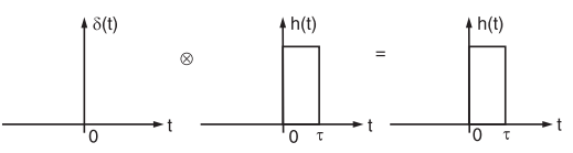
Fig.6 :Convolution of any function with delta function is equal to that function

This means that the width of the pulse in g(t) is determined by the width of h(t) and the sampling instant is determined by delta function.

In fig. 5(b), the starting edge of the pulse represents the point where baseband signal is sampled and width is determined by function h(t). Therefore, g(t) will be expressed as,

This equation has been explained in fig.6.

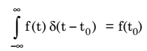
Now, from the property of delta function, we know that for any function f(t)

This property is used to obtain flat top samples. It may be noted that to obtain flat top sampling, we are not applying the above equation directly here i.e., we are applying a modified form of the above equation.

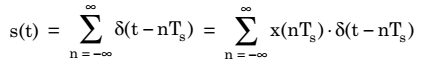
Thus, in this modified equation, we are taking s(t) in place of delta function δ(t).

Observe that δ(t) is a constant amplitude delta function whereas s(t) is a varying amplitude train of impulses. This means that we are taking s(t) which is an instantaneously sampled signal and this is convolved with function h(t).

Therefore, on convolution of s(t) and h(t), we get a pulse whose duration is equal to h(t) only but amplitude is defined by s(t).

Now, we know that the train of impulses may be represented mathematically as,

The signal s(t) is obtained by multiplication of baseband signal x(t) and δT_s(t). Thus,

Now, sampled signal g(t) is given as

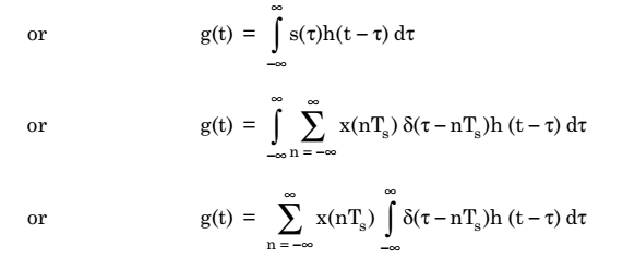
According to shifting property of delta function, we know that

Hence,

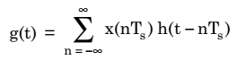
This equation represents value of g(t) in terms of sampled value x(nT_s) and function h(t – nT_s) for flat top sampled signal.

Now, we have

Taking Fourier transform of both sides of above equation, we get

We know that S(f) is given as

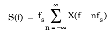
Therefore,

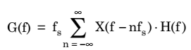
Thus, spectrum of flat top sampled signal:

Fig.8 : (a) Baseband signal x(t), (b) Instantaneously sample signal s(t), (c) Constant pulse width function h(t), (d) Flat top sampled signal g(t) obtained through convolution of h(t) and s(t)